Imagine the universe as a massive program that’s been running since the Big Bang. Every object in it has state (properties) that changes over time according to specific rules (physics laws).

Sound familiar? It should – it’s exactly like any program you’ve written!

📦 The State Variables of Motion

In programming, we manage state with variables. In physics, every moving point mass has three fundamental state variables for 2D motion:

1. Position (x, y) – “Where am I?”

# In code
player_position = {"x": 100, "y": 50}

# In physics
position = (x, y)  # Measured in meters

Think of it as: The object’s coordinates in the world, just like a sprite in a game.

2. Velocity (vx, vy) – “How fast and where am I going?”

# In code
player_velocity = {"vx": 5, "vy": -3}  # Moving right and slightly down

# In physics  
velocity = (vx, vy)  # Measured in meters/second

Think of it as: The change in position per time unit. If position is where you are, velocity is your movement vector.

3. Acceleration (ax, ay) – “How is my velocity changing?”

# In code
player_acceleration = {"ax": 0, "ay": -9.8}  # Gravity pulling down

# In physics
acceleration = (ax, ay)  # Measured in meters/second²

Think of it as: The rate of change of velocity. Forces cause acceleration through Newton’s second law.

🔄 The Universal Game Loop

Every game has a main loop. The universe has one too:

# The Universe's Main Loop (simplified)
while universe_exists:
    for each object in universe:
        # Step 1: Net forces determine acceleration
        net_forces = calculate_all_forces(object)
        acceleration = net_forces / object.mass
        
        # Step 2: Acceleration changes velocity
        object.velocity += acceleration * time_step
        
        # Step 3: Velocity changes position
        object.position += object.velocity * time_step
        
    time += time_step

This is exactly what our projectile simulator does! This loop implements the semi-implicit (symplectic) Euler method – we update velocity first, then position with the new velocity.

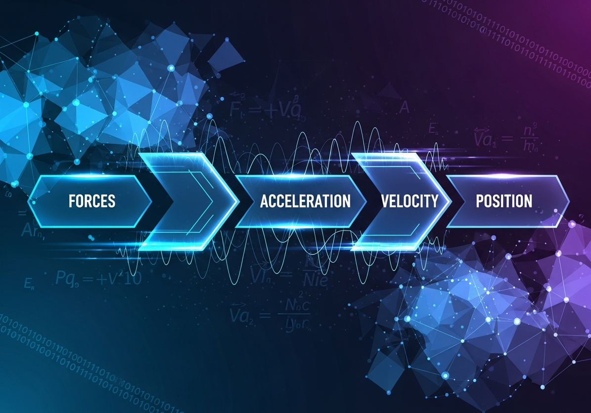
🎯 The Chain of Command

Here’s the hierarchy of how things affect each other:

Forces → Acceleration → Velocity → Position
  ↑           ↑            ↑          ↑
"Push"    "Speeding up"  "Speed"   "Location"

It’s like a cascade of function calls:

• Forces are the input
• Acceleration is the first transformation
• Velocity is the accumulated result
• Position is the final output

💡 Key Insight: Derivatives and Integrals

Remember calculus? (Don’t panic if you don’t!) Here’s all you need to know:

Derivative = Rate of Change

• Velocity is the derivative of position (how position changes)
• Acceleration is the derivative of velocity (how velocity changes)

# In discrete programming terms:
velocity = (position_now - position_before) / time_step
acceleration = (velocity_now - velocity_before) / time_step

Integral = Accumulation

• Position is the integral of velocity (accumulated movement)
• Velocity is the integral of acceleration (accumulated speed change)

# In discrete programming terms:
position_new = position_old + velocity * time_step
velocity_new = velocity_old + acceleration * time_step

🌍 Gravity: The Default Acceleration

Near Earth’s surface, there’s a constant “background process” running in our projectile motion simulations:

G = 9.81  # meters/second² magnitude (varies slightly: ~9.78-9.83)

# Choosing +y as upward, gravity acts downward
acceleration_y = -G  # Downward acceleration due to gravity

Think of gravity as a global constant that affects all objects in our simulation, like a default CSS style that applies to all elements unless overridden.

🧪 Let’s Experiment!

Here’s a simple Python simulation to see state evolution in action:

import matplotlib.pyplot as plt

# Initial state
position = 0
velocity = 20  # m/s upward
g = 9.81  # gravity magnitude
acceleration = -g  # gravity acceleration (downward)

# Storage for plotting
times = []
positions = []
velocities = []

# Simulate for 4 seconds
dt = 0.1  # time step
for step in range(41):
    time = step * dt
    
    # Store current state
    times.append(time)
    positions.append(position)
    velocities.append(velocity)
    
    # Update state (The Physics Engine!)
    velocity = velocity + acceleration * dt
    position = position + velocity * dt
    
    # Stop if hit ground
    if position < 0:
        break

🎓 Key Takeaways

1. Physics is State Management: Objects have position, velocity, and acceleration
2. The Universe Runs a Game Loop: Forces → Acceleration → Velocity → Position
3. Gravity is a Constant: Always there, always ~9.81 m/s² downward near Earth
4. Integration is Accumulation: We add up small changes over time
5. You Already Know This: It's just like updating game sprites!

📚 Programming Parallel

Game programming and physics simulation are remarkably similar:

# Game Programming
class Player:
    def __init__(self):
        self.position = Vector2(0, 0)
        self.velocity = Vector2(0, 0)
        
    def update(self, dt):
        G = 9.81  # gravity magnitude
        self.velocity.y -= G * dt  # Apply gravity (downward)
        self.position += self.velocity * dt  # Update position

# Physics Simulation  
class Projectile:
    def __init__(self):
        self.position = [0, 0]
        self.velocity = [0, 0]
        G = 9.81  # gravity magnitude
        self.acceleration = [0, -G]  # Gravity vector (downward)
        
    def update(self, dt):
        # Semi-implicit Euler integration
        self.velocity[0] += self.acceleration[0] * dt
        self.velocity[1] += self.acceleration[1] * dt
        self.position[0] += self.velocity[0] * dt
        self.position[1] += self.velocity[1] * dt

They're the same picture! 🤝

Understanding physics as state management helps bridge the gap between abstract mathematical concepts and practical programming implementations. The universe really is just running a very sophisticated game loop!